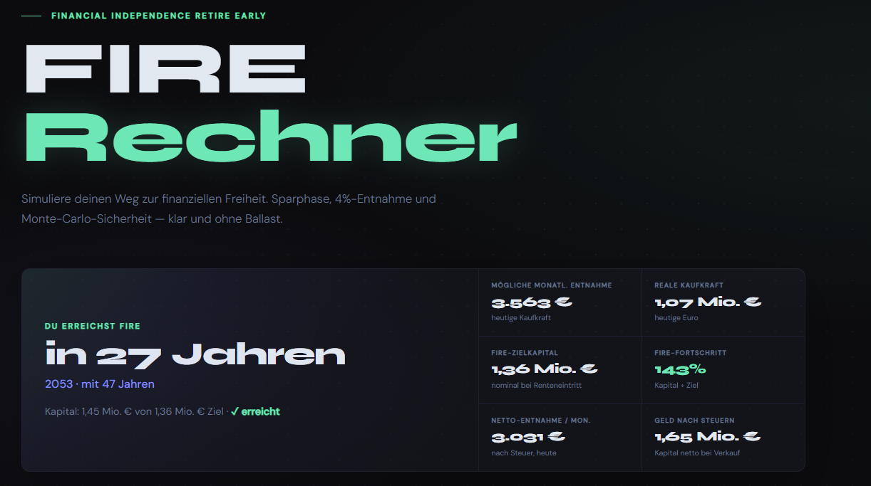
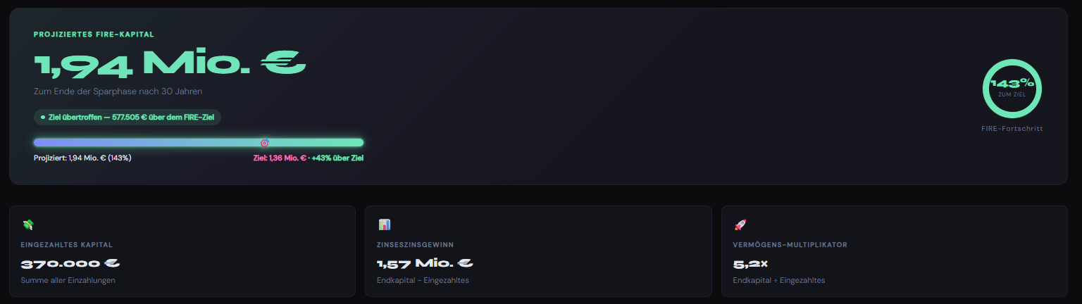
The opening view with the key figures at a glance
About the project
Why I built it
It started with a rather dull Excel sheet where I compared savings rate, returns and time to get a feel for when I might no longer need to work for money. The problem was that every change meant another manual calculation, and it was difficult to see how the individual levers affected each other.
So I turned it into a small web app where every slider updates the charts, table, tax impact and even the probability of running out of money. The deeper I went, the clearer it became that the famous 4% rule does not tell the whole story. Without variation in returns and without German tax effects, any FIRE number can look far safer than it really is.
Features
What the calculator does
- Compound-growth accumulation: Starting capital, monthly savings, expected return, ETF costs and inflation are modelled separately. The results show real purchasing power after costs and inflation.
- FIRE target and 4% rule: The target capital is calculated from the desired withdrawal divided by the withdrawal rate. Adjust the rate to see its effect on the required capital and risk.
- Three withdrawal scenarios: Optimistic, realistic and pessimistic paths run in parallel. Withdrawals are adjusted for inflation and projected to the end of each scenario.
- German tax model: Expert mode accounts for capital gains tax, solidarity surcharge, church tax, the saver’s allowance and partial tax exemptions by fund type.
- Monte Carlo simulation: The calculator generates hundreds of possible paths with adjustable volatility. A P10/P50/P90 fan and the risk of running out of money show the range of outcomes.
- Live charts and annual table: Growth, withdrawals and simulations appear as interactive charts. A year-by-year table adds the underlying values, and every slider triggers a fresh calculation.
Screenshots
A look inside the calculator
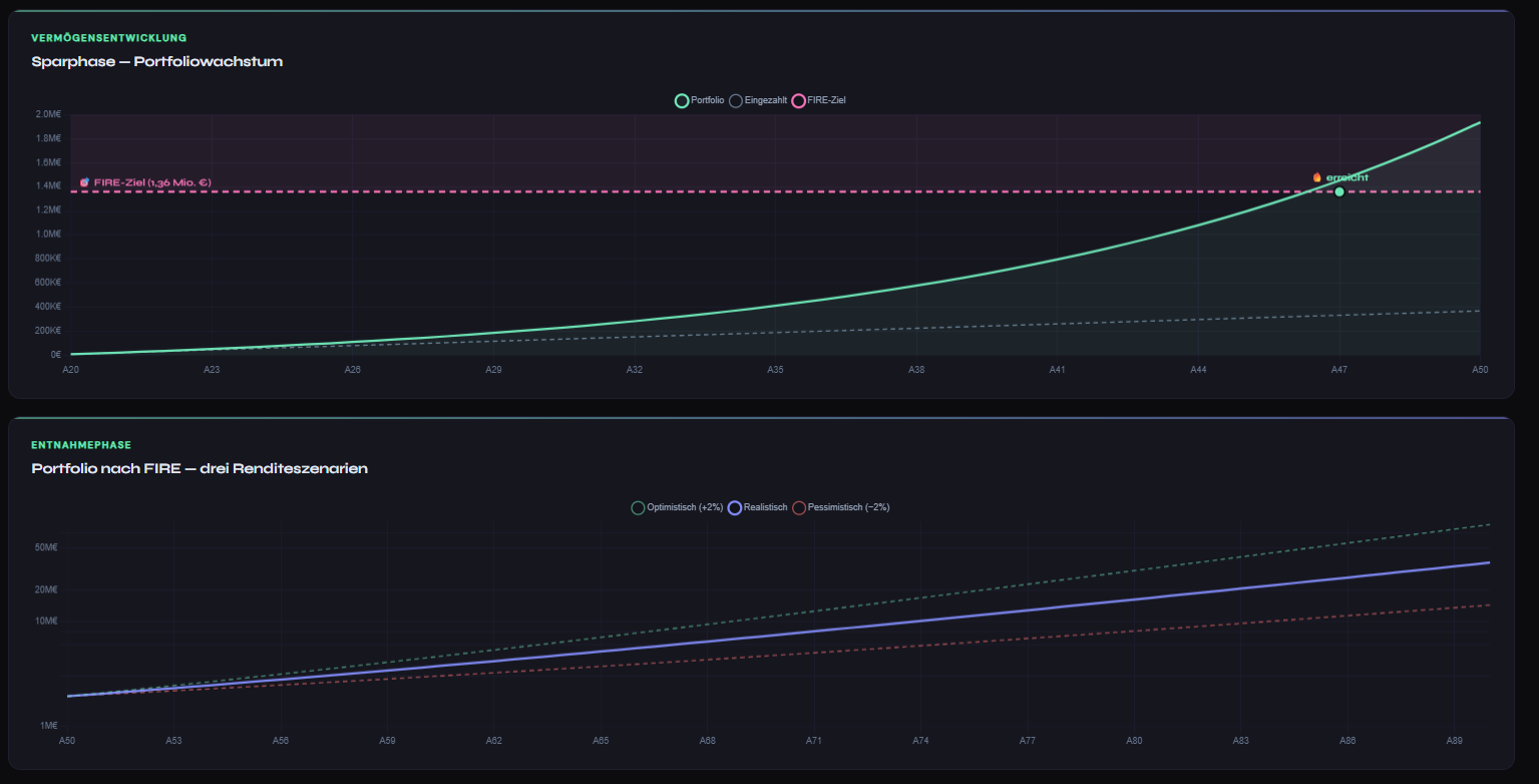
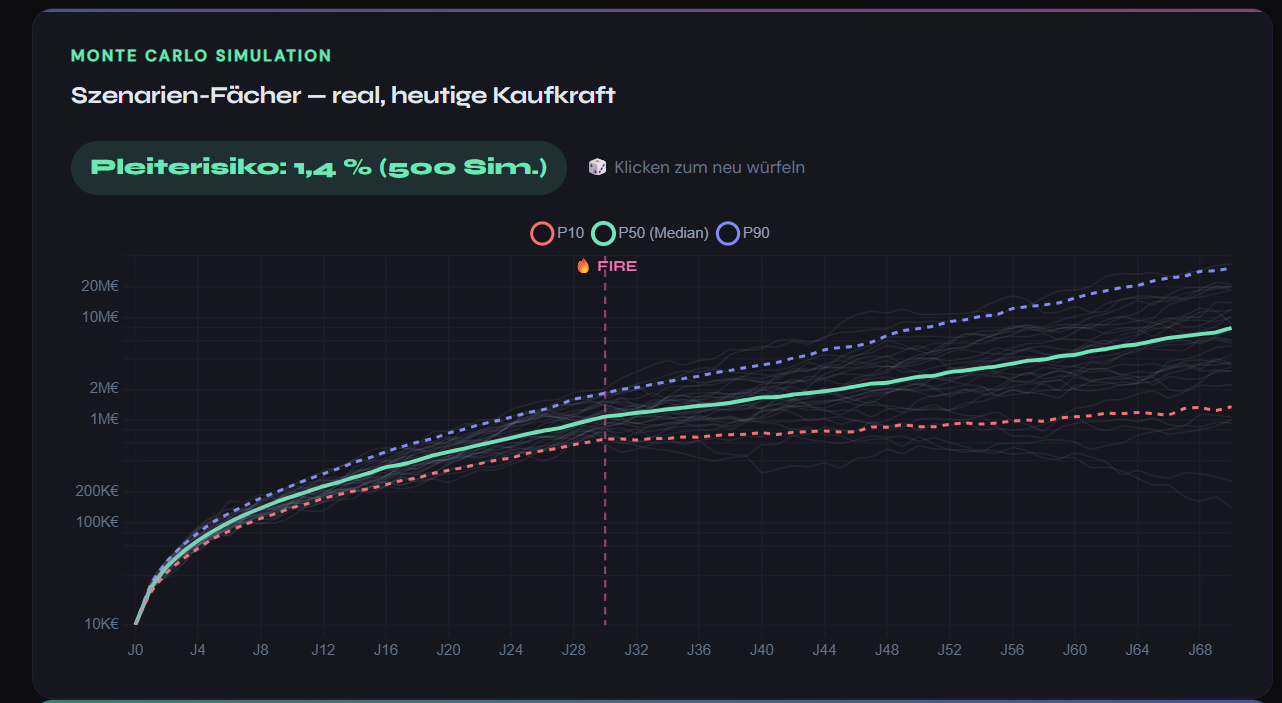
Left: capital path through the accumulation and withdrawal phases | Right: Monte Carlo fan with the risk of running out of money
Technical details
How it works under the hood
The calculator deliberately has no backend. Inputs go straight into JavaScript variables, and every slider change recalculates the full projection: month by month during accumulation and year by year during withdrawals. Chart.js renders the growth, withdrawal and simulation charts, while the design and colours follow the same system as my other projects: a dark background with green and violet accents.
The Monte Carlo simulation draws a random return for each year and run, varying it around the selected expectation. It repeats that process hundreds of times, depending on the chosen number of simulations. A fixed seed keeps the charts stable while sliders are adjusted; an intentional click on the chart starts a new draw.
The tax calculation runs at the FIRE date: gross gains, the partial exemption for the fund type, the saver’s allowance, then capital gains tax, solidarity surcharge and optional church tax. Expert mode can combine several fund types and tax them with their weighted partial exemptions.
Looking back
What I learned
What surprised me most was how much the picture changes when you move from one smooth return assumption to actual variation. A 9% gross return sounds comfortable at first, but inflation, costs and so-called volatility drag leave considerably less in real terms. That made the difference between a deterministic model and a stochastic simulation much clearer.
The tax section showed me how detailed German investment tax law is. Partial exemptions, the saver’s allowance, solidarity surcharge and church tax interact at different points, and getting the order of operations right was more complicated than I expected.
The interface also had to make uncertainty understandable without overwhelming the user with numbers. A percentile fan and a percentage for the risk of running out of money say more than a single figure.